Brusselator
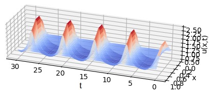
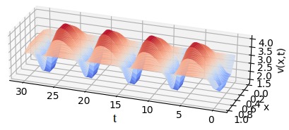
We consider the 1D Brusselator partial differential equation (PDE).
Here we consider a state of the form \(x(y,t)=(u(y,t),v(y,t))\)
where \(y\in \Omega = [0,\ell]\) is the spatial location. The PDE is of the form:
\begin{cases}
\frac{\partial u}{\partial t} = A+u^2v-(B+1)u+\sigma \nabla^2 u\\
\frac{\partial v}{\partial t} = Bu-u^2v+\sigma \nabla^2 v
\end{cases}
with boundary condition:
\(u(0,t)=u(\ell,t)=1\), \(v(0,t)=v(\ell,t)=3\)
and initial condition \(x_0(y)=(u(y,0),v(y,0))\) with:
\(u(y,0)=1+sin(2\pi y)\), \(v(y,0)=3\).
We consider: \(A=1, B=3, \sigma=1/2\), \(\ell =1\).
We transform the PDE into a system of ODEs
by spatial discretization using
a grid of \(N+1\) points with \(N=4\).
We thus consider that we have \(4\) oscillators
of state \(x(y_i,t)\equiv (u(y_i,t),v(y_i,t))\)
with initial conditions \(x(y_i,0)\equiv (u(y_i,0),v(y_i,0))\) (\(i=1,2,3,4\)).
The system of ordinary differential equations for this example is described by:
\begin{equation}
\begin{cases}
\overset{.}{u_1} = A+u_1^2v_1-(B+1)u_1+\sigma (u_0 - 2u_1 + u_2)\\
\overset{.}{v_1} = Bu_1-u_1^2v_1+\sigma (v_0 - 2v_1 + v_2)\\
\overset{.}{u_2} = A+u_2^2v_2-(B+1)u_2+\sigma (u_1 - 2u_2 + u_3)\\
\overset{.}{v_2} = Bu_2-u_2^2v_2+\sigma (v_1 - 2v_2 + v_3)\\
\overset{.}{u_3} = A+u_3^2v_3-(B+1)u_3+\sigma (u_2 - 2u_3 + u_4)\\
\overset{.}{v_3} = Bu_3-u_3^2v_3+\sigma (v_2 - 2v_3 + v_4)\\
\overset{.}{u_4} = A+u_4^2v_4-(B+1)u_4+\sigma (u_3 - 2u_4 + u_5)\\
\overset{.}{v_4} = Bu_4-u_4^2v_4+\sigma (v_3 - 2v_4 + v_5)
\end{cases}
\end{equation}
with \(u_0=u_5=1\) and \(v_0=v_5=3\).
In the results page, we consider a system with uncertainty \(w\in {\cal W}=[-0.05,0.05]\), set of initial conditions \(B(x_0,\varepsilon)\) with \(\varepsilon=0.02\), the time-step used in Euler's method is \(\tau =2\cdot 10^{-4}\), and we take \(T=k\tau\) with \(k=34302\) as an approximate period.
For this example, we check that:
- \(B_{\cal W}((i_0+1)T)\subset B_{\cal W}(i_0T)\) for \(i_0=3\).
The set \({\cal I}_{{\cal W}}\) is an invariant for the system with uncertainty, and contains the limit cycle (LC).
The computation time is 48 seconds.
Results
Source code
Readme
Biped
Example 1:
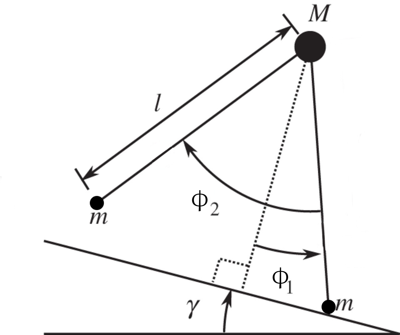
We consider a simple model of biped walker, seen as
a hybrid oscillator.
The figure opposite shows a schematic diagram of the model, where
\(l\) is the length of the legs; \(M\) and \(m\) are the masses of the hip and the foot,
respectively; \(\phi_1\) and \(\phi_2\) specify the angles of the swing and support legs and \(\gamma\) is the angle of the slope.
This model exhibits a stable limit-cycle oscillation for appropriate parameter values that corresponds to periodic movements of the legs.
The model has a unique mode (\(U=\{1\}\)) and a continuous state variable \(\textbf{x}(t) = (\phi_1(t), \overset{.}{\phi_1}(t), \phi_2 (t), \overset{.}{\phi_2} (t))^\top\) .
The dynamics is described by:
\begin{equation}
\textit{f}(\textbf{x}) = \begin{pmatrix}
\overset{.}{\phi_1} \\
sin(\phi_1-\gamma)\\
\overset{.}{\phi_2}\\
sin(\phi_1 - \gamma) + \overset{.}{\phi_1^{2}} sin \phi_2 - cos (\phi_1 - \gamma) sin \phi_2
\end{pmatrix}
\end{equation}
\begin{equation}
Reset(\textbf{x}) = \begin{pmatrix}
-\phi_1\\
\overset{.}{\phi_1}sin(2\phi_1)\\
-2\phi_1\\
\overset{.}{\phi_1 }cos 2\phi_1 ( 1 - cos 2\phi_1 )
\end{pmatrix}
\end{equation}
\begin{equation}
Guard(\textbf{x})=0 \equiv (2\phi_1 - \phi_2 =0\ \wedge \phi_2< -\delta) ,
\end{equation}
We consider: \(\gamma=0.009\), \(\delta=0.1\) and initial condition \(x(0) = (0.200236, -0.199756, 0.40055, -0.01585) \).
In the results page, we consider a system without uncertainty (\(w=0\)), set of initial conditions \(B(x_0,\varepsilon)\) with \(\varepsilon=0.001\), the time-step used in Euler's method is \(\tau =2\cdot 10^{-4}\), and we take \(T=k\tau\) with \(k=19417\) as an approximate period.
For this example, we check that:
- \(B_{\cal W}((i_0+1)T)\subset B_{\cal W}(i_0T)\) for \(i_0=0\).
The set \({\cal I}_{{\cal W}}\) is an invariant for the system with uncertainty, and contains the limit cycle (LC).
The computation time is 24 seconds.
Results
Source code
Readme
Biped
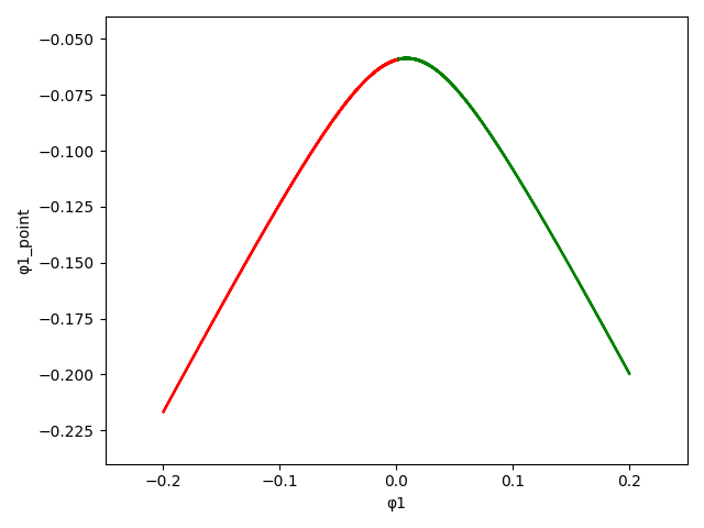
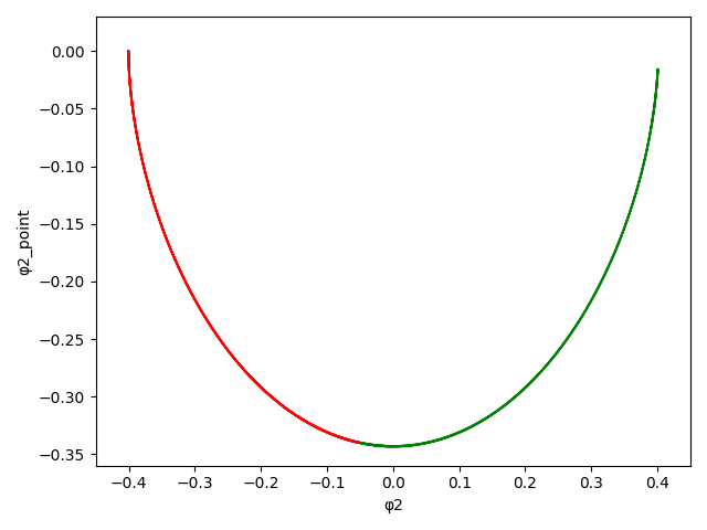
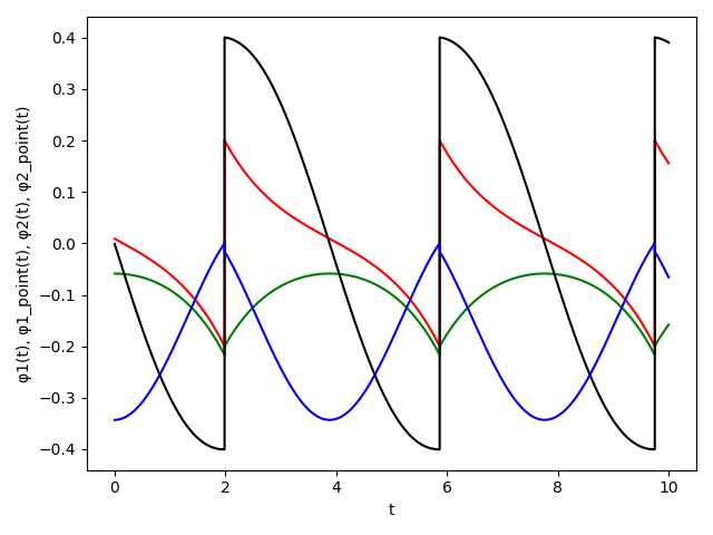
Example 2:
We repeat the same experience as in Example 1 (Biped),
we consider here: \(\gamma=0.009\), \(\delta=0.1\), initial condition \(x(0) = (0.009, -0.05869, -0.0009629, -0.3432) \)
and a system without uncertainty (\(w=0\)), set of initial conditions \(B(x_0,\varepsilon)\) with \(\varepsilon=0.01\), the time-step used in Euler's method is \(\tau =2\cdot 10^{-5}\), and we take \(T=k\tau\) with \(k=194129\) as an approximate period.
For this example, we check that:
- \(B_{\cal W}((i_0+1)T)\subset B_{\cal W}(i_0T)\) for \(i_0=0\).
The set \({\cal I}_{{\cal W}}\) is an invariant for the system with uncertainty, and contains the limit cycle (LC).
The computation time is 212 seconds.
Results
Source code
Readme
Biped
Example 3:
We repeat the same experience as in Example 1 (Biped),
we consider here: \(\gamma=0.009\), \(\delta=0.1\) and initial condition \(x(0) = (0.009, -0.05869, -0.0009629, -0.3432) \)
and a system with uncertainty \(w\in {\cal W}=[-0.00005,0.00005]\), set of initial conditions \(B(x_0,\varepsilon)\) with \(\varepsilon=0.01\), the time-step used in Euler's method is \(\tau =2\cdot 10^{-5}\), and we take \(T=k\tau\) with \(k=194129\) as an approximate period.
For this example, we check that:
- \(B_{\cal W}((i_0+1)T)\subset B_{\cal W}(i_0T)\) for \(i_0=4\).
The set \({\cal I}_{{\cal W}}\) is an invariant for the system with uncertainty, and contains the limit cycle (LC).
The computation time is 409 seconds.
Results
Source code
Readme
Van der Pol
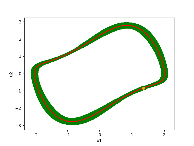
Example 1:
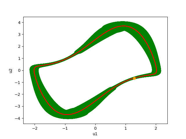
Consider the Van der Pol (VdP) system \(\Sigma_p\) of dimension \(n=2\) with parameter \(p\geq 0\),
and initial condition in \(B_0=B_{\cal W}(x_0,\varepsilon)\)
for some \(x_0\in\mathbb{R}^2\) and \(\varepsilon>0\):
\begin{equation*}
\begin{cases}
du_1/dt=u_2\\
du_2/dt=p u_2 -p u_1^2u_2-u_1\\
\end{cases}
\end{equation*}
Consider now the system \(\Sigma'\) with uncertainty \(w_0\in{\cal W}_0\):
\begin{equation*}
\begin{cases}
du_1/dt=u_2\\
du_2/dt=(p_0+w_0) u_2 -(p_0+w_0) u_1^2u_2-u_1\\
\end{cases}
\end{equation*}
with \(p_0=1.1\).
Each solution of \(\Sigma_p\) with \(p\in[p_0-0.02,p_0+0.02]=[1.08,1.12]\)
and initial condition \(x_0\) is thus a particular solution of the system \(\Sigma'\) with uncertainty
\(w\in {\cal W}_0=[-0.02,0.02]\) and set of initial conditions \(B(x_0,\varepsilon_0)\).
With: \(x_0=(u_1(0),u_2(0))=(1.35473686, -0.843734)\), initial radius \(\varepsilon_0=0.1\), \(\tau=1/1000\) and \(T_0=6.746=6746\tau\).
For this example, we check that:
- \(B_{\cal W}((i_0+1)T)\subset B_{\cal W}(i_0T)\) for \(i_0=0\).
The set \({\cal I}_{{\cal W}}\) is an invariant for the system with uncertainty, and contains the limit cycle (LC).
The computation time is 748 seconds.
Results
Source code
Readme
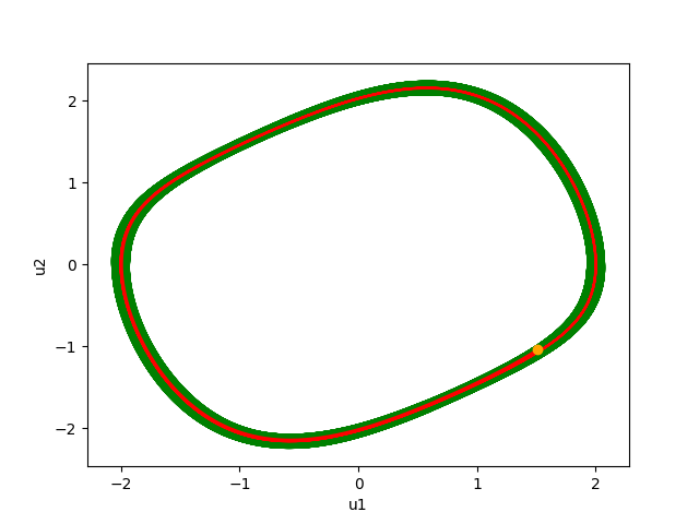
Van der Pol
Example 2:
We repeat the same experience as in Example 1 (Van der Pol),
but for the value of the parameter \(p_1 = 0.4\), the amplitude
of uncertainty \(w\in {\cal W}_1=[-0.01,0.01]\), and initial radius \(\varepsilon_1=0.1\).
Each solution of \(\Sigma_p\) with \(p\in[p_1-0.01,p_1+0.01]=[0.39,0.41]\)
and initial condition \(x_0\) is
now a particular solution of \(\Sigma'\) with uncertainty
\(w\in {\cal W}_1=[-0.01,0.01]\) and set of initial conditions \(B(x_0,\varepsilon_1)\).
With: \(x_0=(u_1(0),u_2(0))=(1.35473686, -0.843734)\), \(\tau=1/1000\) and \(T_1=6.347=6347\tau\).
For this example, we check that:
- \(B_{\cal W}((i_0+1)T)\subset B_{\cal W}(i_0T)\) for \(i_0=2\).
The set \({\cal I}_{{\cal W}}\) is an invariant for the system with uncertainty, and contains the limit cycle (LC).
The computation time is 603 seconds.
Results
Source code
Readme
Van der Pol
Example 3:
We repeat again the same experience as in Example 1 (Van der Pol),
but for the value of the parameter \(p_2 = 1.9\), the amplitude
of uncertainty \(w\in {\cal W}_2=[-0.025,0.025]\), and initial radius \(\varepsilon_2=0.1\).
Each solution of \(\Sigma_p\) with \(p\in[p_2-0.025,p_2+0.025]=[1.875,1.925]\)
and initial condition \(x_0\) is
now a particular solution of \(\Sigma'\) with uncertainty
\(w\in {\cal W}_2=[-0.025,0.025]\) and set of initial conditions \(B(x_0,\varepsilon_2)\).
With: \(x_0=(u_1(0),u_2(0))=(1.35473686, -0.843734)\), \(\tau=1/1000\) and \(T_2=7.53=7530\tau\).
For this example, we check that:
- \(B_{\cal W}((i_0+1)T)\subset B_{\cal W}(i_0T)\) for \(i_0=2\).
The set \({\cal I}_{{\cal W}}\) is an invariant for the system with uncertainty, and contains the limit cycle (LC).
The computation time is 761 seconds.
Results
Source code
Readme