\(\delta\) function:
Consider a differential system with bounded uncertainty
of the form \(\{\dot{x}(t)=f(x(t),w(t))\}\) where \(w\) belongs to the bounded uncertainty set \({\cal W}\).
We suppose that for all \(y_1,y_2\in {\cal S}\) (\({\cal S}\) is a bounded region \({\cal S} \subset \mathbb{R}^d\) containing the solutions of the system) and \(w_1,w_2\in {\cal W}\)
there exist constants \(\lambda\in\mathbb{R}\) and \(\gamma\in\mathbb{R}_{\geq 0}\)
satisfying the equation:
\begin{multline}\label{eq:H1}
\langle f(y_1,w_1)-f(y_2,w_2), y_1-y_2\rangle
\\
\leq
\lambda\|y_1-y_2\|^2 + \gamma \|y_1-y_2\|\|w_1-w_2\|
\end{multline}
Recall that \(\lambda\) has to be computed in the absence of uncertainty
(\({\cal W}=0\)). The additional constant \(\gamma\) is used for taking into account
the uncertainty \(w\).
Given \(\lambda\), the constant \(\gamma\) can be computed itself
using a nonlinear optimization solver. Instead of computing them globally
for \(S\), it is advantageous to compute \(\lambda\) and \(\gamma\) locally depending on the subregion of \(S\) occupied by the system state during a considered interval of time.
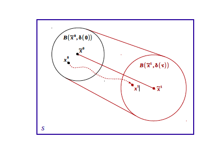
Consider a point \(x_0\in {\cal S}\) and a point \(y_0\in {\cal B}(x_0,\varepsilon)\).
Let \(x(t;y_0)\) be the exact solution of the system \(\frac{dx(t)}{dt}=f(x(t),w(t))\) with bounded uncertainty \({\cal W}\) and initial condition \(y_0\),
and \(\tilde{x}(t;x_0)\) the Euler approximate solution of the system \(\frac{dx(t)}{dt}=f(x(t),0)\) without uncertainty (\({\cal W}=0\)) with initial condition \(x_0\).
We have, for all \(w(\cdot) \in {\cal W}\) and \(t\in[0,\tau]\):
\begin{equation}
\|x(t;y_0)-\tilde{x}(t;x_0)\|\leq \delta_{\varepsilon,{\cal W}}(t).
\end{equation}
with:
- if \(\lambda <0\),
\begin{multline}
\delta_{\varepsilon,{\cal W}}(t) =
\left( \frac{C^2}{-\lambda^4} \left( - \lambda^2 t^2 - 2 \lambda t + 2 e^{\lambda t} - 2 \right) \right. \\
+ \left. \frac{1}{\lambda^2} \left( \frac{C \gamma |{\cal W}|}{-\lambda} \left( - \lambda t + e^{\lambda t} -1 \right) \right. \right. \\ + \left. \left. \lambda \left( \frac{\gamma^2 (|{\cal W} |/2)^2}{-\lambda} (e^{\lambda t } - 1) + \lambda \varepsilon^2 e^{\lambda t} \right) \right) \right)^{1/2}
\end{multline}
- if \(\lambda >0\),
\begin{multline}
\delta_{\varepsilon,{\cal W}}(t) = \frac{1}{(3\lambda)^{3/2}} \left( \frac{C^2}{\lambda} \left( - 9\lambda^2 t^2 - 6\lambda t + 2 e^{3\lambda t} - 2 \right) \right. \\
+ \left. 3\lambda \left( \frac{C \gamma |{\cal W}|}{\lambda} \left( - 3\lambda t + e^{3\lambda t} -1 \right) \right. \right. \\
+ \left. \left. 3\lambda \left( \frac{\gamma^2 (|{\cal W} |/2)^2}{\lambda} ( e^{3\lambda t } - 1) + 3\lambda \varepsilon^2 e^{3\lambda t} \right) \right) \right)^{1/2}
\end{multline}
- if \(\lambda = 0\),
\begin{multline}
\delta_{\varepsilon,{\cal W}}(t)=
\left( {C^2} \left( - t^2 - 2 t + 2 e^{ t} - 2 \right) \right. \\
+ \left. \left( {C \gamma |{\cal W}|} \left( - t + e^{ t} -1 \right) \right. \right. \\ + \left. \left. \left({\gamma^2 (|{\cal W} |/2)^2} ( e^{ t } - 1) + \varepsilon^2 e^{ t} \right) \right) \right)^{1/2}
\end{multline}
where \(|{\cal W}|\) is the diameter of \({\cal W}\) (maximum distance between 2 points of \({\cal W}\)).