Robust

About image About image About image

Biochemical process

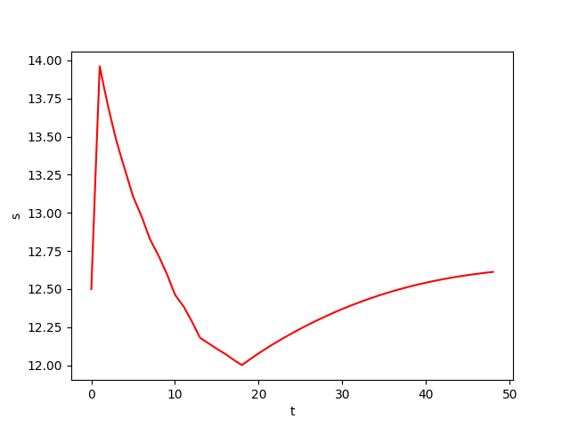
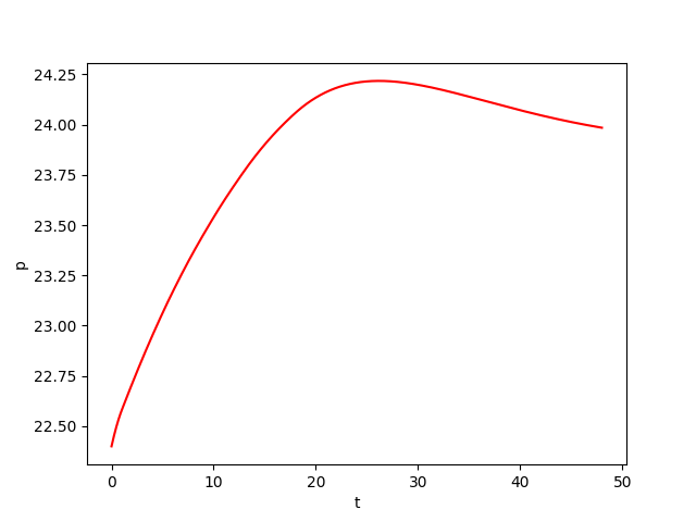
We consider a biochemical process model \(Y\) of continuous culture fermentation. Let \(Y = (X, S, P) \in \mathbb{R}^3\) satisfies the differential system: \begin{equation*} \begin{cases} \overset{.}{X}(t) = -D X(t) + \mu(t) X(t)\\ \overset{.}{S}(t) = D \big( S_f(t) - S(t) \big) - \frac{\mu(t)X(t)}{Y_{x/s}}\\ \overset{.}{P}(t) = -D P + \big( \alpha\mu(t) + \beta \big) X(t)\\ \end{cases} \end{equation*}

where \(X\) denotes the biomass concentration, \(S\) the substrate concentration, and \(P\) the product concentration of a continuous fermentation process. The model is controlled by \(S_f \in [S_f^\mathit{min}, S_f^\mathit{max}]\). While the dilution rate \(D\), the biomass yield \(Y_{x/s}\) , and the product yield parameters \(\alpha\) and \(\beta\) are assumed to be constant and thus independent of the actual operating condition, the specific growth rate \(\mu : \mathbb{R} \rightarrow \mathbb{R}\) of the biomass is a function of the states:

\begin{equation*} \mu(t) = \mu_m\frac{\left( 1-\frac{P(t)}{P_m}\right) S(t)}{K_m + S(t)+\frac{S(t)^2}{K_i}} \end{equation*}

The goal is to maximize the average productivity presented by the cost function:

\begin{equation*} J_k = \frac{1}{T}\int^T_0DP(t)dt \end{equation*}

Results Source code Readme

Spin

We consider a 1/2 spin particle system \(X\). Let \(X = (x, y, z) \in \mathbb{R}^3\) satisfies the differential system:

\begin{equation*} \overset{.}{X(t)} = A(\vec{\omega}) X(t) + D \end{equation*}

where \(D = (0, 0, \gamma)^\top)\) and \(A(\vec{\omega})\) is a \(3 \times 3\) matrix:

\begin{equation*} A(\vec{\omega}) = \begin{pmatrix} -\Gamma & -\omega & \omega_y(t)\\ \omega & -\Gamma & -\omega_x(t)\\ -\omega_y(t) & \omega_x(t) & -\gamma \\ \end{pmatrix} \end{equation*}

with \(\vec{\omega}(t) = (\omega_x(t), \omega_y(t)) \). The model is controlled by \(\vec{\omega}(t)\) where \(\omega_y(t) = 0\). The goal is to maximize the normalized figure of merit:

\begin{equation*} F_{opt} = \frac{1}{\sqrt{1+T_c}}\sqrt{x(T_c)^2 + y(T_c)^2} \end{equation*}

where \(T_d\) and \(T_c\) denote the detection time (fixed by the experimental setup) and the control time, respectively.

Results Source code Readme
Services image
Services image Services image

Van Der Pol

We consider Van Der Pol system with: \begin{equation*} \begin{cases} \overset{.}{x}(t) = 10 (y + x - 1/3 x^3)\\ \overset{.}{y}(t) = b_0 - x - 0.75y \end{cases} \end{equation*} In the right, we present some simulations of \(y(x(t))\) first with \(b_0=0.3\) and then with \(b_0=\sqrt(2)/3\).
In the two cases, the blue curve designates the simulations of \(y(x(t))\), the red zone indicates the expansive area (\(\lambda>0\)) and the black point shows the fixed point at the saddle-node bifurcation.
In the first figure (when \(b_0=0.3\)), x and y form a limit cycle. In the second figure (when \(b_0=\sqrt(2)/3\approx0.471\) at the saddle­‐node (SN) bifurcation), the limit cycle collides with the fixed black point \(\approx (0.97,-0.66)\) and disappears.

Results Source code Readme
Design: TemplateMo