Example 1: Biochemical Process
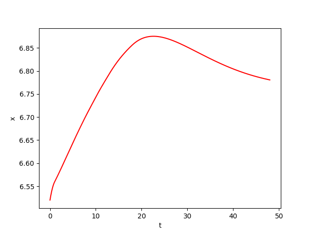
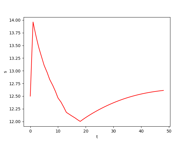
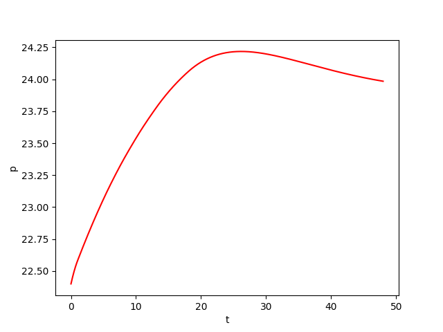
We consider a biochemical process model \(Y\) of continuous culture fermentation. Let \(Y = (X, S, P) \in \mathbb{R}^3\) satisfies the differential system: \begin{equation*} \begin{cases} \overset{.}{X}(t) = -D X(t) + \mu(t) X(t)\\ \overset{.}{S}(t) = D \big( S_f(t) - S(t) \big) - \frac{\mu(t)X(t)}{Y_{x/s}}\\ \overset{.}{P}(t) = -D P + \big( \alpha\mu(t) + \beta \big) X(t)\\ \end{cases} \end{equation*} where \(X\) denotes the biomass concentration, \(S\) the substrate concentration, and \(P\) the product concentration of a continuous fermentation process. The model is controlled by \(S_f \in [S_f^\mathit{min}, S_f^\mathit{max}]\). While the dilution rate \(D\), the biomass yield \(Y_{x/s}\) , and the product yield parameters \(\alpha\) and \(\beta\) are assumed to be constant and thus independent of the actual operating condition, the specific growth rate \(\mu : \mathbb{R} \rightarrow \mathbb{R}\) of the biomass is a function of the states:\begin{equation*} \mu(t) = \mu_m\frac{\left( 1-\frac{P(t)}{P_m}\right) S(t)}{K_m + S(t)+\frac{S(t)^2}{K_i}} \end{equation*}
The goal is to maximize the average productivity presented by the cost function:\begin{equation*} {\cal J}_{z_0,\varepsilon}(x(\cdot),u(\cdot))= \frac{1}{T}\int^T_0DP(t)dt \end{equation*}
with \(x(\cdot)=(X(\cdot),S(\cdot),P(\cdot))\) and \(x(0)\in B(z_0,\varepsilon)\) while satisfying the constraint on the state \(X\):\begin{equation} \frac{1}{T}\int^T_0X(t)dt\leq 5.8 \end{equation}
In the following experiences presented in "Results" page (the bottom below), we consider a codomain \([28.7, 40]\) of the original continuous control function \(S_f(\cdot)\) which is discretized into a finite set \(U\), for the needs of our method. After discretization, \(S_f(\cdot)\) is a piecewise-constant function that takes its values in the finite set \(U\) made of 2 values uniformly taken in \(\{28.7, 40\}\). The function \(S_f(\cdot)\) changes (possibly) its value every \(\tau\) seconds. We take: \(z_0=(6.52, 12.5, 22.40)\), \(\varepsilon=0\), \(\tau = 3\), \(\Delta t=\tau/100\), \(T= 48\), \(K=T/\tau=16\). We consider an additive disturbance \(d\) with \(d(\cdot)\in {\cal D}= [-0.05,0.05]\). We perform 3 experiences:- We randomly pick one sample over every \(100\) possible controls, which gives \(2^{16}/100 \approx 655\) samples.
- We randomly pick one sample over every \(10\) possible controls, which gives \(2^{16}/10 \approx 6,554\) samples.
- We consider all the possible controls, which gives \(2^{16} = 65,536\) samples.
- We get: \({\cal K}_{z_0,\varepsilon}(u^*)=3.1618\) (the constraint on the state \(X\) is satisfied since \(\frac{1}{T}\int^T_0X(t)dt = 5.782 \leq 5.8\)). The CPU computation time of this example is 7 seconds.
- We get: \({\cal K}_{z_0,\varepsilon}(u^*)=3.1667\) (the constraint on the state \(X\) is satisfied since \(\frac{1}{T}\int^T_0X(t)dt = 5.794 \leq 5.8\)) The CPU computation time of this example is 18.69 seconds.
- We get: \({\cal K}_{z_0,\varepsilon}(u^*)=3.1677\) (the constraint is satisfied since \(\frac{1}{T}\int^T_0X(t)dt = 5.7995 \leq 5.8\)). The CPU computation time of this example is 200 seconds.