Phase transitions of composition schemes: Mittag-Leffler and mixed Poisson distributions
Webpage accompanying the article arXiv:2103.03751, by Cyril Banderier, Markus Kuba, and Michael Wallner
October 2021
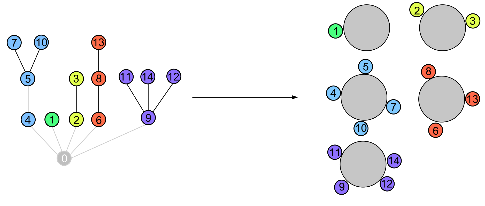
Many combinatorial structures are enumerated by the scheme $F(z)=G(H(z)) \times M(z)$.
For a structure $\mathcal F$, the underlying structure $\mathcal G$ is called its "skeleton" or its "core".
Some natural questions are: What is the typical shape of a structure $\mathcal F$?
What is the typical size of its core?
I.e., in a big structure of size $n$, under the uniform distribution amongst all structures $\mathcal F$ of size $n$,
- what is the number $X_n$ of $\mathcal H$-blocks,
- what is the number $X_{n,j}$ of $\mathcal H$-blocks of any given size $j$?
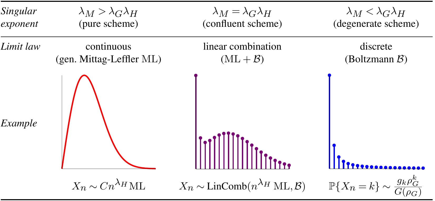
The corresponding limit laws
are quite involved when one has a critical composition scheme,
i.e. if the functions $G$ and $H$ become simultaneously non-analytic:
the radius of convergence of $G$ is $H(\rho)$, where $\rho$ is the dominant singularity of $H$.
(If the composition is not critical, the situation is easier to handle: one typically gets a Gaussian limit, or a discrete distributions;
see the book "Analytic combinatorics" by Flajolet and Sedgewick).
In the critical case, we show that the limit laws are more complicated: they involve Boltzmann distributions, generalized Mittag-Leffler distributions,
some linear combinations of these, and mixed Poisson distributions!
 |
|
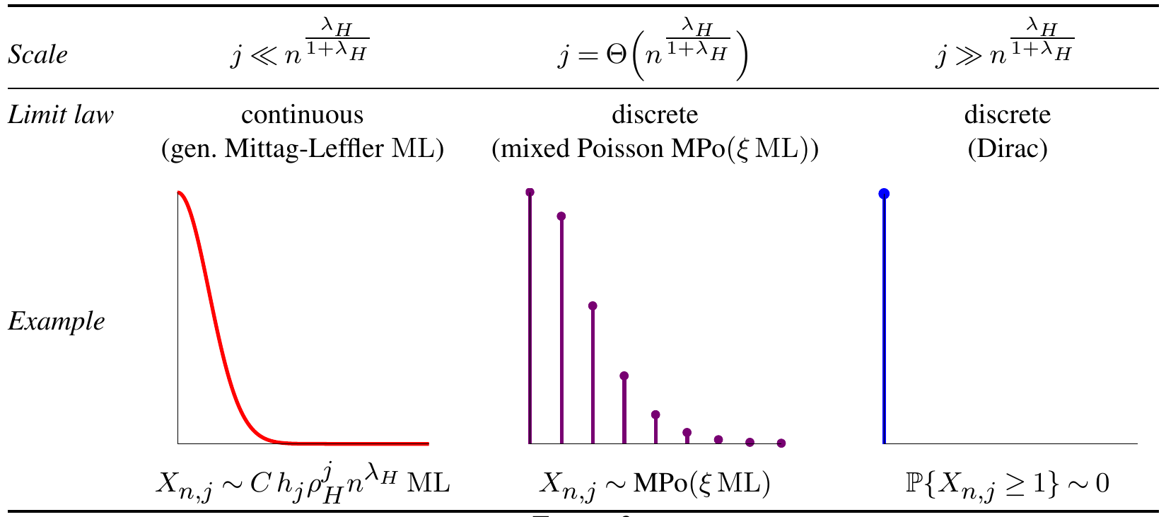 |
The parameters of these distributions depend
in a crucial way on the singular exponent $\lambda_H$ of $H(z)$, coming from the Puiseux expansion
$H(z) = H(\rho) + C.(1-z/\rho)^{\lambda_H} +... $
As many structures have a singular exponent 1/2 (this follows e.g. from the Drmota-Lalley-Woods theorem), our results also show why one so often can get a phase transition
at size $j=n^{1/3}$.
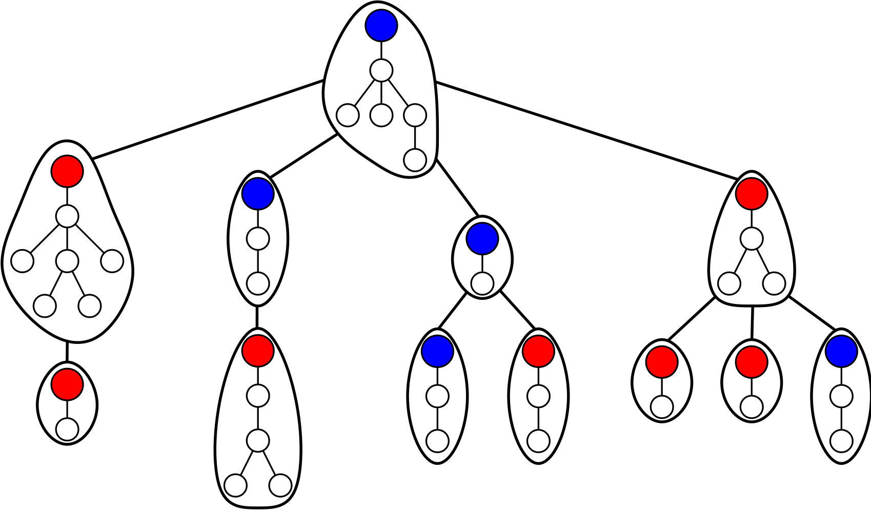
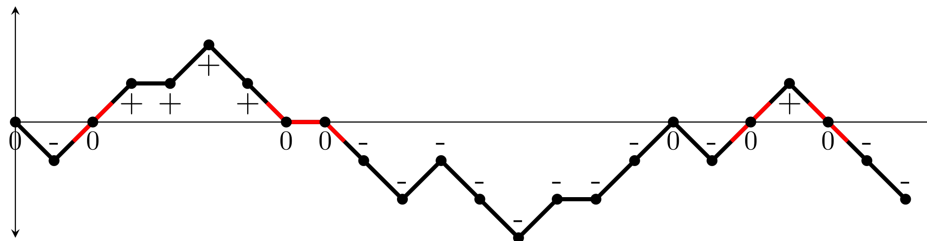
Here are some examples of statistics/combinatorial structures handled by these critical schemes (see Section 6 of our article):
nodes of a given color in supertrees, returns to zero and sign changes in random walks, node degrees in increasing trees,
table occupation in the Chinese restaurant model, number of balls of a given color in Pólya urns.
 | |  | 
|  |
Let us now illustrate the corresponding distributions for different values of their parameters:


