We give below a list of benchmarks of hybrid systems, showing the different functions and options offered by HYMITATOR.
For each case study, we give the source file (.hym), the command to launch HYMITATOR, the log output by the tool (.log), the set of states reached in a textual form (.states), and some graphical outputs.
Navigation Benchmark
For this benchmark, HYMITATOR is used in mode reachability, viz., to compute the set of reachable states.
The command used is as follows:
HYMITATOR NAV01.hym -mode reachability -plot x y -limits x 0 3 -limits y 0 3 -fancy
(and similarly for NAV04)
-plot x y is an additional facility of HYMITATOR that automatically outputs the set of trajectories in 2 dimensions (for variables x and y). The "-limits x 0 3" option gives the bounds for the graphics.
| Model | Log | States | Trace set | Trajectories |
|---|---|---|---|---|
| NAV01 | NAV01.log | NAV01.states | NAV01.jpg | NAV01.png |
| NAV04 | NAV04.log | NAV04.states | NAV04.jpg | NAV04.png |
Water Tank
For this benchmark, HYMITATOR is used for a CEGAR analysis with predicate abstraction.
The command used is as follows:
HYMITATOR tank.hym -mode cegar -fancy
| Model | Log | States | Trace set |
|---|---|---|---|
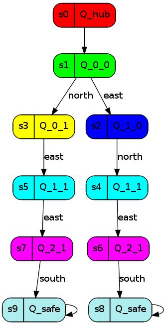
| tank | tank.log | tank.states | tank.jpg |
Fischer’s Mutual Exclusion Protocol
For this benchmark, HYMITATOR is used to perform parameter synthesis using the inverse method.
The command used is as follows:
HYMITATOR fischer.hym fischer.pi0 -inclusion
The -inclusion option asks HYMITATOR to consider a fixpoint where all states are included (in the sense of constraint inclusion) into previously encountered states, rather than strict equality.
| Model | Reference valuation | Log | States | Trace set |
|---|---|---|---|---|
| fischer | fischer.pi0 | fischer.log | fischer.states | fischer.jpg |
Jumping Frog
For this benchmark, HYMITATOR is used to perform parameter synthesis using the inverse method.
The command used is as follows:
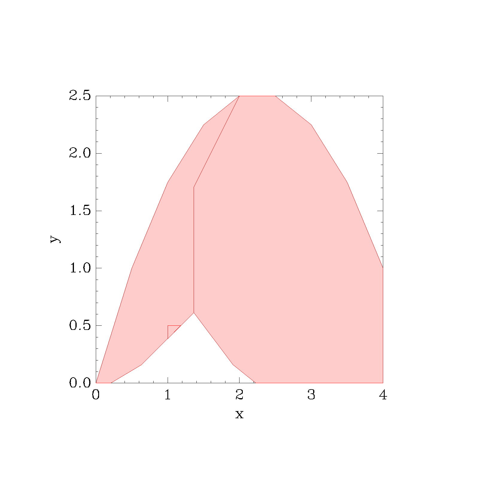
HYMITATOR jump.hym jump.pi0 -inclusion -plot x y -limits x 0 4 -limits y 0 2.5 -fancy
Again, we use the facilities offered by HYMITATOR to output the trajectories in a graphical form.
| Model | Reference valuation | Log | States | Trace set | Trajectories |
|---|---|---|---|---|---|
| jump | jump.pi0 | jump.log | jump.states | jump.jpg | jump.png |
Scheduling Case Studies
We present in the following table a list of case studies computed using the inverse method, as implemented in HyMITATOR. These case studies are not strictly speaking hybrid, but are parametric timed automata equipped with stopwatches.
We give from left to right the name of the case study (with a link to the HyMITATOR model), the reference, the reference valuation file pi0, the number |A| of automata in parallel, the number |X| of clocks, the number |P| of parameters, the number |S| of states computed, the number |T| of transitions computed, the number n of iterations of the inverse method, the number |K| of inequalities within the resulting constraint K, the computation time t in seconds (excluding the generation of the graphical outputs), the file containing the resulting constraint, the file containing the description of all states, and the trace set given under a graphical form.
All experiments were performed on a machine equipped with an Intel Core 2 processor with 2.93GiHz and 2GiB RAM, running operating system Ubuntu 11.10 (32 bits version).
| Case study | Reference | V0 | |A| | |X| | |P| | t | Log | Cartography |
|---|---|---|---|---|---|---|---|---|
| BB04 | [BB04] | bb.v0 | 5 | 7 | 10 | 66s | bb.log | bb.png |
Description of the Case Studies
We can group our case studies in five classes.
- The FPs and EDFs case studies are composed of three cyclic tasks that need to be performed on a single machine.
Therefore, the machine has to choose which task is active when several tasks are requiring computation.
This is done in two ways, either with a Fixed Priority (FP) scheduler or an Earliest Deadline First scheduler (EDF).
These case studies are being studied in the framework of the joint project Roscov between LSV and an industrial partner [Soulat12].
For every FP scheduling example, each task tau_i has the following parameters: an offset O_i, a Wost Case Execution Time (WCET) C_i, a period T_i and a deadline to achieve a given goal (modeled by an extra automaton).
For every EDF scheduling example, each task tau_i has the following parameters: an offset O_i, a WCET C_i, a period T_i, a deadline D_i to achieve each task, and a deadline to achieve a given goal (modeled by an extra automaton). - The Task Chain case study does not use cyclic tasks but instead has a 4 task chain and a concurrent 3 task chain. Each task in a chain cannot start until the previous one has not terminated. Each task in each chain has a given fixed priority. A scheduler assigns which task has the computational time with a FP policy.
- CPR08 and LPPRC10 are two-cyclic-tasks problem with an EDF scheduler.
- AM02, LA02 2*5, LA02 3*5 case studies are problems of preemptive job-shop scheduling. AM02 is an example with two jobs on three machines; LA02 2*5 (resp. LA02 3*5) corresponds to the example from [LA02] (with 10 jobs on 5 machines) with here only the 2 (resp. 3) first jobs on 5 machines.
- BB04 case study corresponds to a three task example from [BB04, Section III, table 1]. It is an FP scheduling problem with three cyclic tasks on one machine. This case study actually uses the behavioral cartography algorithm (see [AF10]).
Algorithms used
All case studies use the merging technique introduced in [AFS12].
For all case studies except three, the standard Inverse Method algorithm was used. To execute HYMITATOR, use:
> HYMITATOR case_study.imi case_study.pi0 -merge
For the LA02 2*5 and LA02 3*5 case studies, we made use of Algorithm IMincl (introduced in [AS11]). To execute HYMITATOR, use:
> HYMITATOR case_study.imi case_study.pi0 -merge -inclusion
For the BB04 case study, the cartography algorithm (introduced in [AF10], and iteratively calling the inverse method) was used. To execute HYMITATOR, use:
> HYMITATOR bb.imi bb.v0 -merge -mode cover [-no-dot -no-log]
Full details about models and results are available in [Soulat12].
References
- [AM02]
- Yasmina Abdeddaïm and Oded Maler. Preemptive job-shop scheduling using stopwatch automata. In TACAS'02, pages 113–126, 2002.
- [AS11]
- Étienne André and Romain Soulat. Synthesis of Timing Parameters Satisfying Safety Properties. In RP’11, pages 31–44, 2011.
- [BB04]
- Enrico Bini and Giorgio C. Buttazzo. Schedulability analysis of periodic fixed priority systems. IEEE Trans. Computers, 53(11):1462–1473, 2004.
- [CPR08]
- Cimatti, Palopoli and Ramadian. Symbolic Computation of Schedulability Regions Using Parametric Timed Automata. In RTSS’08.
- [LPPRC10]
- Thi Thieu Hoa Le, Luigi Palopoli, Roberto Passerone, Yusi Ramadian, Alessandro Cimatti. Parametric Analysis of Distributed Firm Real-Time Systems: A Case Study. In ETFA’2010: 1-8.
- [LA02]
- http://bach.istc.kobe-u.ac.jp/csp2sat/jss/
- [SGL97]
- Jun Sun, Mark K. Gardner, and Jane W. S. Liu. Bounding Completion Times of Jobs with Arbitrary Release Times, Variable Execution Times, and Resource Sharing. IEEE Trans. Softw. Eng., 1997.
- [Soulat12]
- Romain Soulat. Scheduling with IMITATOR: Some Case Studies. Research Report, Laboratoire Spécification et Vérification, March 2012.
Contact
In case you meet any problem in performing these experiments (or your own models), please contact us.


